Evaluating the Representation Space of Diffusion Models via Self-Supervised Principles
1University of Michigan · 2Ohio State University · *Equal contribution
TL;DR. Diffusion models can be evaluated and monitored from within, using the geometry of their own learned representations — no labels, no sampling, no external networks needed.
Diffusion models are also representation learners
Diffusion models have achieved remarkable generative results, but their internal representations are also powerful: features extracted from a frozen diffusion backbone at the right noise level perform competitively with dedicated self-supervised learning (SSL) methods on downstream classification, segmentation, and correspondence tasks.
This raises a natural question: if diffusion models are strong representation learners, can we use the quality of their representations as a window into their generative behavior?
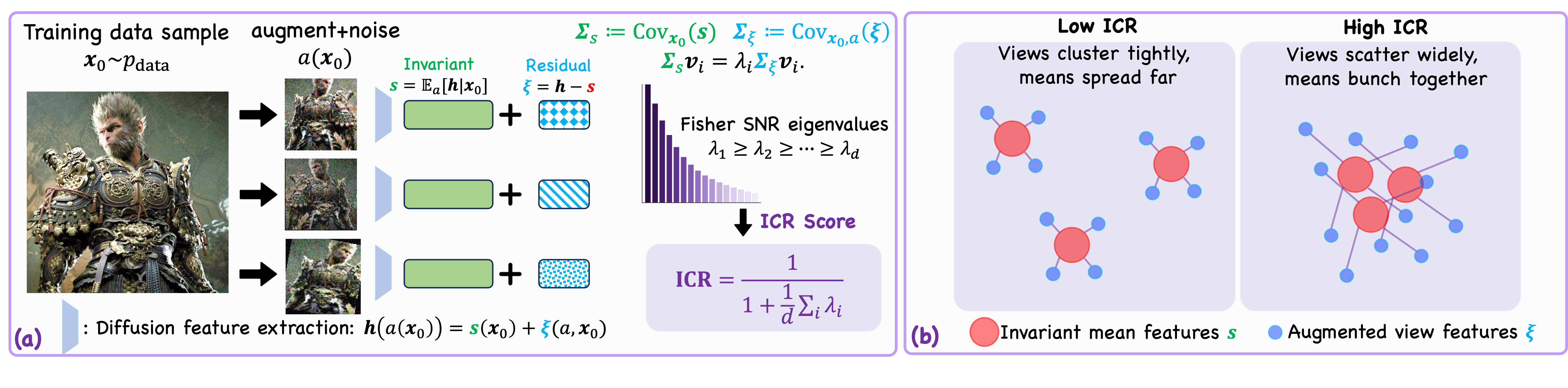
Overview of the \(\mathrm{ICR}\) Framework. Each training image is augmented and passed through the diffusion feature extractor, decomposing representations into an invariant component \(\bm{s}\) and a residual \(\bm{\xi}\); their covariances define \(\mathrm{ICR}\).
What makes a good representation?
Modern SSL methods are built on two complementary principles. First, representation invariance: features of different augmented views of the same image should remain stable. Second, representation expansion: features should spread out across the embedding space, avoiding collapse and preserving distinct image identities.
For diffusion models, these properties are not explicitly optimized — only a denoising objective is. Yet we find they emerge implicitly, and measuring them offers a natural diagnostic for diffusion models.
We decompose each representation into two components. For a training image \(\bm{x}_0\) and a random perturbation \(a\) (data augmentation + diffusion noise):
\[\bm{s}(\bm{x}_0) := \mathbb{E}_a\!\left[\bm{h}(a(\bm{x}_0))\mid \bm{x}_0\right], \qquad \bm{\xi}(a,\bm{x}_0) := \bm{h}(a(\bm{x}_0)) - \bm{s}(\bm{x}_0).\]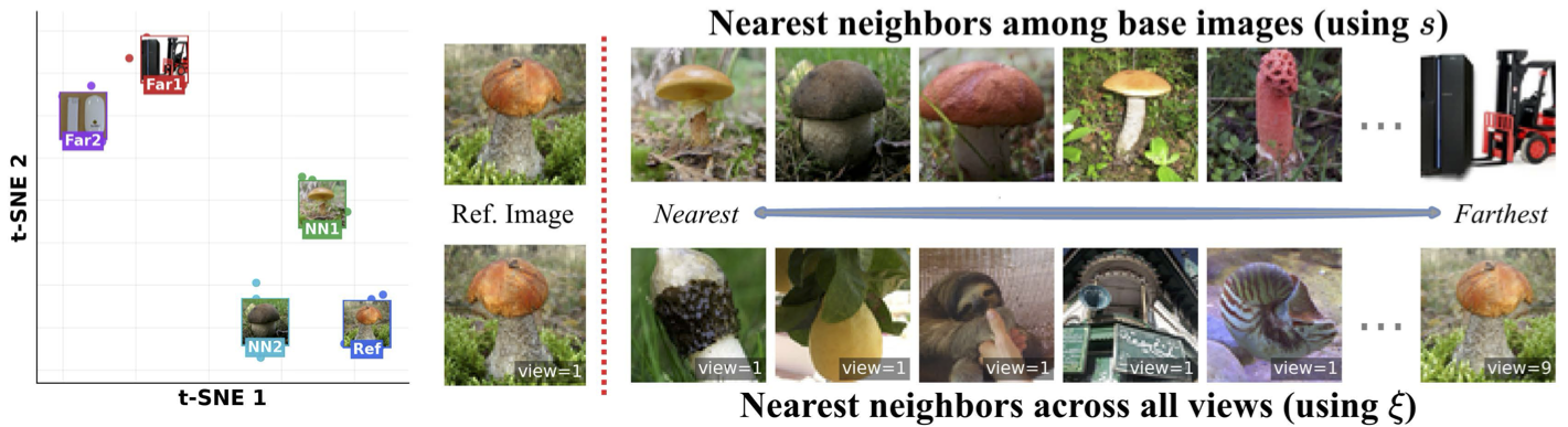
Invariant vs. residual components. Nearest neighbors via the invariant component \(\bm{s}\) are semantically related to the query; neighbors via the residual \(\bm{\xi}\) are not.
Here \(\bm{s}\) is the invariant component — stable across noisy and augmented views — and \(\bm{\xi}\) is the residual component capturing view-specific variation. The total feature covariance then decomposes cleanly as \(\bm{\Sigma}_h = \bm{\Sigma}_s + \bm{\Sigma}_\xi\).
The Invariant Contamination Ratio (ICR)
To summarize the health of the representation space in a single trackable scalar, we introduce the Invariant Contamination Ratio (ICR). We solve the generalized eigenproblem \(\bm{\Sigma}_s \bm{v}_i = \lambda_i \bm{\Sigma}_\xi \bm{v}_i\), where each eigenvalue \(\lambda_i\) measures the invariant signal-to-noise ratio along a :
This follows the same generalized eigenstructure as classical Fisher Linear Discriminant Analysis, where \(\bm{\Sigma}_s\) and \(\bm{\Sigma}_\xi\) play roles analogous to between-class and within-class covariances — with each individual image acting as its own "class."
ICR approaches 0 when the invariant component dominates across all Fisher directions (a clean, structured representation), and approaches 1 when residual variation floods the space (a contaminated one). Crucially, ICR is entirely label-free and computed from training features alone — no generation, external encoders, or held-out data.
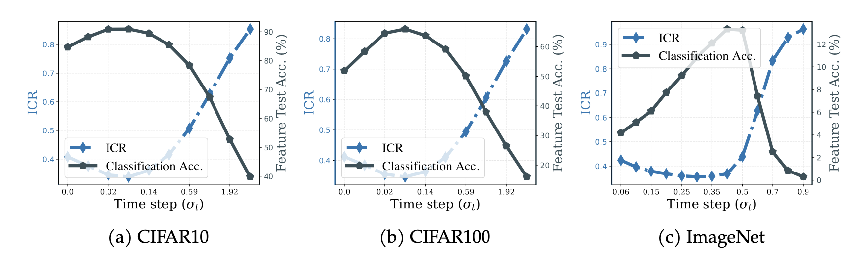
ICR predicts downstream performance across noise levels. The noise levels that minimize ICR coincide with those that maximize linear classification accuracy — a semantic window where representations are strongest.
A semantic window in the noise schedule
The diffusion noise schedule creates a family of representations indexed by noise level \(\sigma_t\). At very low noise, representations are entangled with fine-grained, augmentation-specific details. At very high noise, they collapse toward uninformative Gaussian structure. In between, an intermediate range yields the richest semantic structure.
ICR identifies this range automatically. Across CIFAR10, CIFAR100, and ImageNet, the ICR curve is U-shaped and attains its minimum around the noise levels where linear probe accuracy peaks. This gives a simple, label-free rule for selecting the best noise scale for diffusion features (no downstream classifier required during selection).
Tracking generalization and memorization during training
We fix an intermediate noise scale and track ICR as training progresses. The behavior splits cleanly by data regime.
In the data-rich regime, ICR and FID decrease simultaneously throughout training. As the model better approximates the underlying distribution, its internal features shift toward stable, low-dimensional structure. ICR captures this improvement from the inside, without the need to generate new samples.
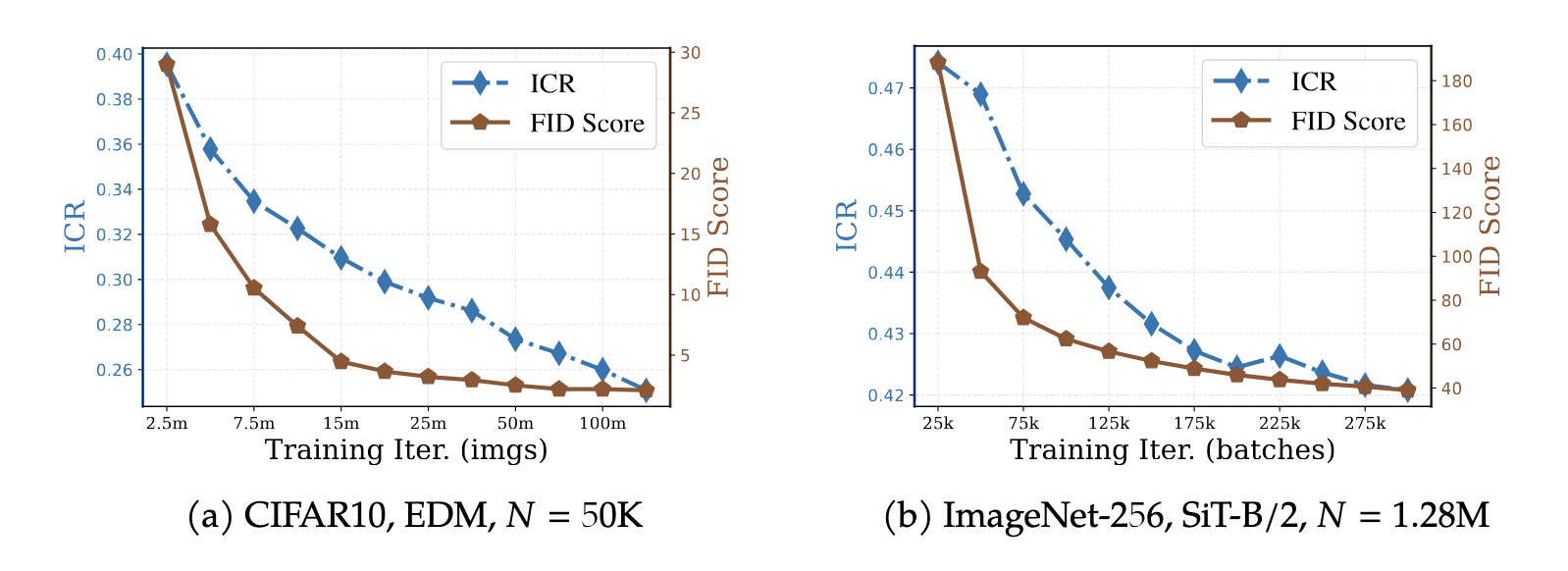
ICR tracks FID in the data-rich regime. Both decrease monotonically, reflecting improving representation invariance and generation quality in parallel.
In the data-limited regime, the picture changes sharply. ICR follows a clear U-shaped trajectory: it first decreases as the model learns genuine structure, then rises again as the model begins fitting sample-specific idiosyncrasies. Recent work has documented this — but prior detection methods either require large numbers of generated samples or rely on FID, which is known to be unreliable for memorization detection.
The early learning phenomenon in diffusion models — where image quality initially improves before the model begins to memorize — has been documented across several recent works. See for exmaple Li et al. (2024) and Bonnaire et al. (2026).
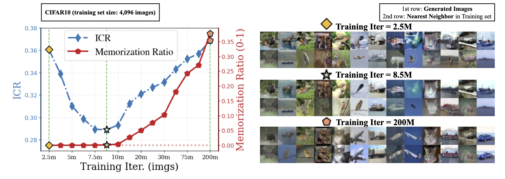
ICR anticipates memorization. The memorization ratio remains near zero around the ICR minimum and rises only afterward — making ICR a practical, label-free early stopping signal.
The ICR minimum marks the transition point: beyond it, the model gradually starts to memorize individual training samples rather than learning shared semantic structure. The nearest neighbors of the invariant component track this transition qualitatively — they are semantically meaningful near the ICR minimum and degrade on both sides.
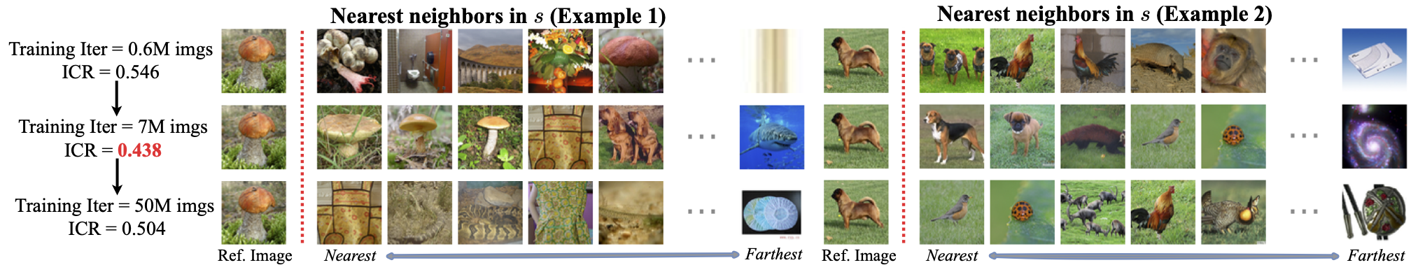
Nearest neighbors track the training transition. At the ICR minimum (middle row), retrieved neighbors are more semantically close than the early and late stages, where ICR is larger.
What drives feature expansion?
ICR is a relative measure; it does not directly reveal how total representation energy evolves. Examining the traces \(\mathrm{Tr}(\bm{\Sigma}_s)\) and \(\mathrm{Tr}(\bm{\Sigma}_\xi)\) separately also shows a difference between training regimes. In the data-rich setting, growing feature capacity is predominantly devoted to the invariant component \(\bm{\Sigma}_s\). In the data-limited setting, once the limited semantic structure has been largely extracted, further feature expansion is dominated by the residual component \(\bm{\Sigma}_\xi\) — the model starts "filling up" with noise rather than signal.
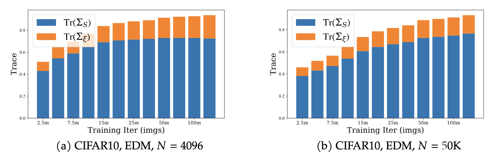
Feature expansion is driven by invariant structure when data are abundant, and by residual variation when data are scarce and invariant structure signal is saturated.
A unified perspective
Our results suggest that diffusion models can be monitored and understood alternatively through the geometry of their own learned representations. ICR provides an intrinsic training-time signal that is:
- Label-free — no class annotations or external encoders needed.
- Sample-free — computed from training features, not generated images.
- Sensitive — detects the onset of memorization.
- Interpretable — rooted in a clean invariant/residual decomposition with a direct signal-to-noise interpretation.
This work is part of a growing effort to bridge self-supervised representation learning and generative diffusion modeling, showing that insights from one enrich our understanding of the other.